BEAMTAP Simulations.

BEAMTAP - Broadband and Efficient Adaptive Method for Time-delay Array Processing.

Click here to jump to the beginning of the BEAMTAP home page.

The following figures were generated by a simulation tool created as a widget based GUI under the IDL programming language. This tool was developed with the objective of simulating the optical implementation of the BEAMTAP algorithm for true-time delay adaption of large antenna arrays for detection of broadband signals in the presence of multiple strong broadband jammers. This work is being developed under a MURI sponsored by the Office of the Secretary of Defense (DDR & E) managed by Dr. William Miceli of the Office of Naval Research.

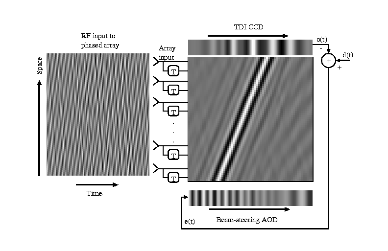
Diagram describing the simulation of the BEAMTAP optical architecture. The input signal is represented by the leftmost figure. At every time-step a instantaneous slice of the input is detected by the antenna arrays and it is forward propagated through the adaptive weights (center figure) and detected and accumulated at the TDI-CCD (upper figure). The instantaneous output o(t) is subtracted from the instantaneous desired signal d(t), generating the error signal e(t), which is fed through the AOD (lower figure). An outer-product between the AOD signal and a delayed version of the input is used to adapt the weights, producing the resulting cross-correlation seen in the center figure.

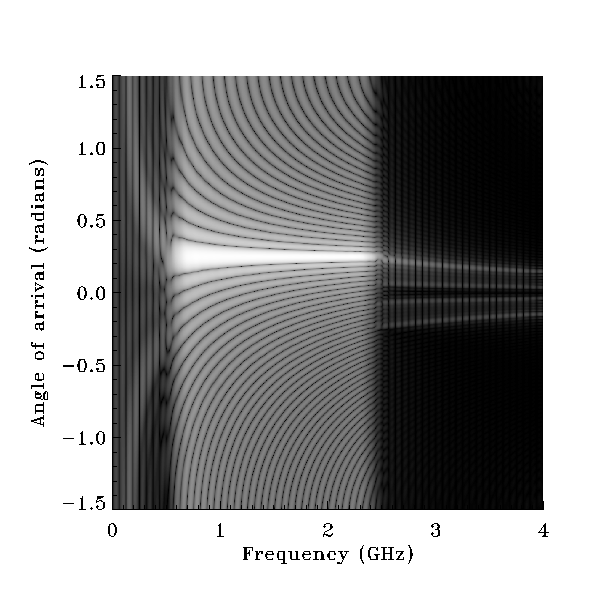
Fourier-space representation of the input signals used in the computer simulation of the optical implementation of the BEAMTAP algorithm. The input signals are selected in order to test the system's spatio-temporal jammer nulling capacity over a diversified signal environment. The desired signal is a broadband gaussian chirp. Jammer 1 is a broadband filtered gaussian noise and jammer 2 is a single frequency sine wave.

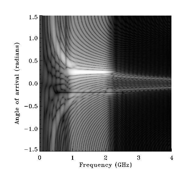
Beamforming: Receptivity pattern of the simulated system after adaptation when only the desired signal is present at the input, demonstrating squint-free true time-delay beam-forming. Notice that system response (main lobe) spans the whole input signal bandwidth.

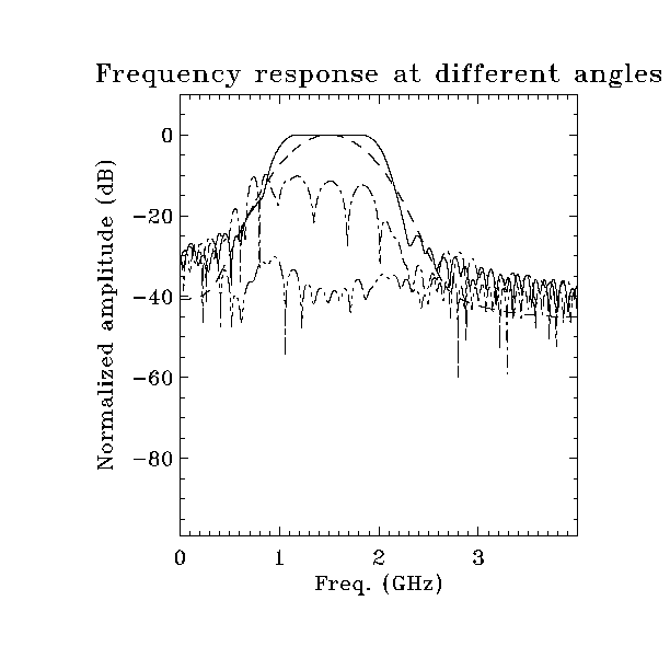
Jammer nulling: Receptivity pattern of the simulated system after adaptation when the desired signal and strong jammers are present at the input, demonstrating squint-free jammer suppression with deep nulls. Notice nulls at jammer locations and slight reduction in the bandwidth of the system response to the desired signal.

Jammer nulling: Plots of the receptivity pattern at angles of arrival of interest. Solid line: 0.25 radians. Beamforming at the angle of arrival of the desired signal. Dashed line: fequency spectrum of the desired gaussian pulse. Dash-dot: 0.2 radians. Null at the narrowband frequency (0.8GHz). Dash-dot-dot: -0.2 radians. Wide null at the broadband jammer bandwidth (from 0.5GHz to 2.5GHz). Notice Wiener filtering, where the bandwidth of the frequency response at the angle of arrival of the desired signal has been reduced in order to optimally compensate for the narrowband jammer, maximizing the signal to interference plus noise (SINR) ratio.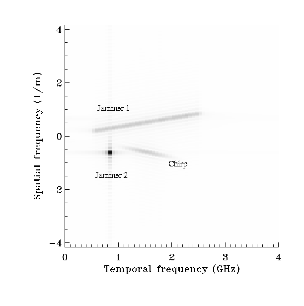

Back to my home page.

Last Modified: 24/Mar/2002